Reading Snowflake Query Profiles to Diagnose Slow Queries

Two Snowflake queries with the character-for-character same SQL can finish one in four seconds and the other in four minutes, and the query text will never tell you why. SQL is a request, not a record of what happened: it says what result the user wants, not which micro-partitions got scanned, whether the warehouse spilled to disk, or whether the query sat in a queue behind three other jobs. Snowflake's optimizer compiles that request into a physical execution plan, and the plan's shape often bears little resemblance to the order the SQL was written in, because the optimizer reorders, pushes down filters, and picks join strategies based on data it has already profiled. The Query Profile is the tool that closes that gap. It shows what Snowflake actually did, not what was asked for, and reading it well turns slow-query diagnosis into something closer to a checklist than a guessing game.

Where to find the Query Profile and what it retains

The path is short: Snowsight, then Monitoring, then Query History, then select a query and open its Query Profile tab. Every executed query sitting in Query History has a Profile link attached to it, and clicking it opens the visual DAG that's the subject of most of this piece.

One constraint matters more than it should: profiles are retained for 14 days after a query completes. That's not a lot of runway if a post-incident review gets scheduled for the following sprint, so anyone doing retrospective diagnosis on a slow batch job needs to pull the profile before it ages out, not after someone finally asks about it in a meeting.

On first open, four panels show up. Query Plan is the DAG itself, the visual map of operators. Most Expensive Nodes pre-sorts the operations by resource consumption, which is a reasonable place to start if the graph looks intimidating. Profile Overview breaks total execution time into phases, processing time versus I/O time and so on. Statistics lists the harder numbers: partitions accessed, bytes scanned, spill figures. Between the four, there's rarely a need to go hunting elsewhere for a first pass.

How the DAG is structured

The graph is a Directed Acyclic Graph, which is a formal way of saying arrows only point one direction and never loop back. Nodes are physical operators, things like a table scan, a join, a grouping step, an ordering step. Arrows are data flow: how many rows moved from one operator into the next.

Execution runs bottom to top. The lowest nodes are almost always TableScans, pulling data out of storage, and the single node at the very top is typically the Result. Reading upward along those arrows is the fastest way to spot where row counts did something unexpected, ballooning after a join, or barely shrinking after a filter that should have cut the set down hard.

The tree shows only operators that consumed more than 1 percent of total execution time. Smaller operations get collapsed out of view. This keeps the graph from turning into visual noise, but it also means the Profile is already doing some editorial work on the reader's behalf, surfacing the operators that matter and hiding the rest.

The five signals the Profile surfaces

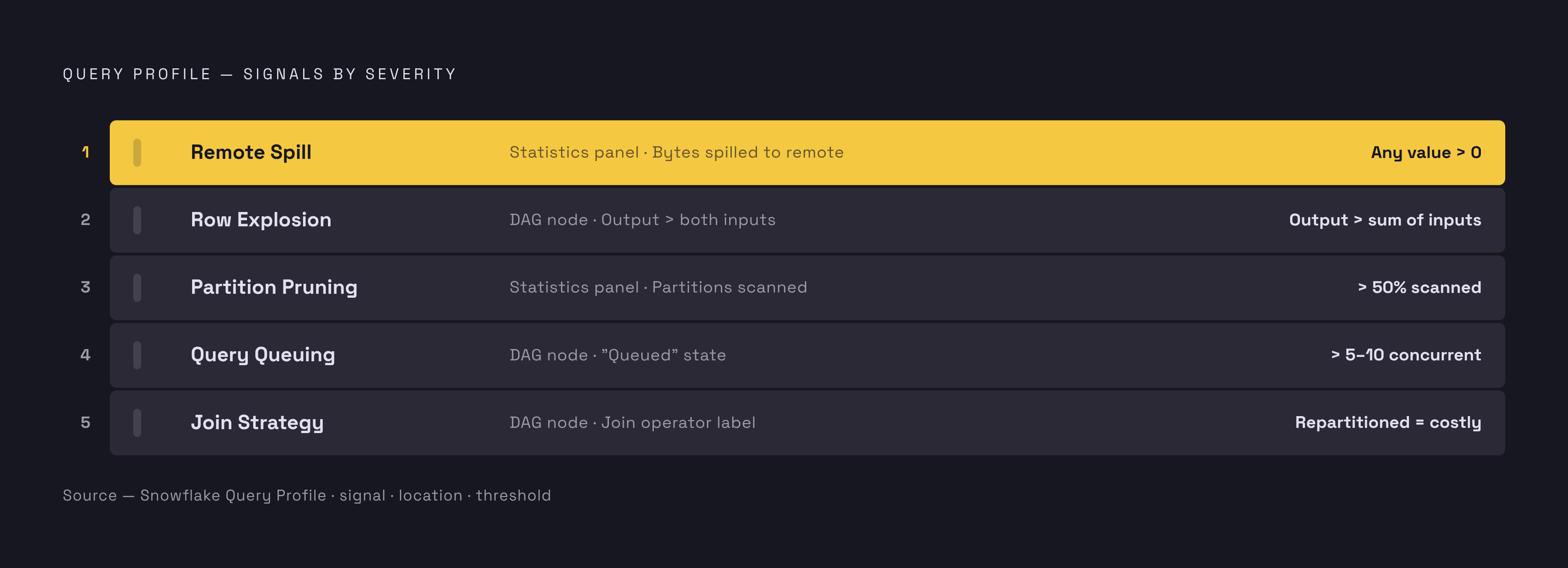
Most diagnostic work in the Profile comes down to five things. Some show up in the DAG directly, others live in the Statistics panel, but together they cover the overwhelming majority of "why is this slow" questions.

Partition pruning ratio: Snowflake stores table data in micro-partitions, immutable compressed columnar files, each one carrying the min/max value of every column inside it. When a query filters on a column, the optimizer checks that metadata first and skips any partition that can't possibly satisfy the filter, without ever reading the actual data. A well-pruned query might skip the large majority of a table's partitions. A poorly pruned one reads the whole table regardless of the filter. In the TableScan node, look at partitions scanned against partitions total: crossing 50 percent scanned is worth investigating. The usual offender is a function wrapped around a clustered column in the WHERE clause, something like WHERE TO_DATE(created_at) = '2024-01-01', because Snowflake can't evaluate min/max ranges through a function call, so pruning quietly stops working even though the column itself is clustered.

Spill to local and remote storage: when an operation's intermediate result set outgrows the memory available on the warehouse, Snowflake writes the overflow to local disk. If local disk isn't enough either, it spills further, out to remote cloud storage (S3, Azure Blob, GCS, depending on the cloud). Remote spill causes a dramatic slowdown, the single worst thing that can happen to a query's runtime from a memory standpoint. The Statistics panel shows "Bytes spilled to remote" directly, and any number above zero deserves attention. The fix is one of two things: size the warehouse up so there's more memory to work with, or restructure the query, smaller intermediate aggregations, narrower sorts, so it needs less memory from the start.

Row explosion from joins is when a join's output row count is larger than both of its inputs combined, and it's the easiest failure to spot visually because the row count on the arrow leaving the Join node is just obviously bigger than what went in. The usual causes are a join condition that's wrong, a join condition that's missing entirely (a Cartesian product in disguise), or a one-to-many relationship nobody accounted for when writing the query. The Profile also shows the join strategy: a broadcast join, where a small dimension table gets copied to every node, is cheap; a repartitioned join across two large tables is expensive, and the DAG will show which one Snowflake picked.

Query queuing happens if the warehouse is already saturated: new queries wait rather than run, and that wait time shows up in the Profile Overview and in query history metadata. More than 5 to 10 concurrent queries competing for the same warehouse, or queries that regularly sit in a "Queued" state, points to a warehouse that's undersized for how many people are hitting it at once. This distinction matters for diagnosis: a query that sits in queue for a long stretch but runs quickly once it starts does not have a slow-query problem. It has a concurrency problem, and no amount of query rewriting will fix that.

What to do when the Profile points to a structural problem rather than a query fix

Not every slow query gets fixed by editing the query. Sometimes the Profile shows that the warehouse itself, or the table layout underneath it, causes the actual constraint.

Scaling decisions split into two directions, and the Profile tells you which one applies. Scale up, meaning move to a larger warehouse size, when queries are CPU- or memory-bound: heavy aggregations, complex transformations, anything showing remote spill. Scale out, meaning add a multi-cluster warehouse, when the Profile shows queuing rather than long processing time, since more clusters mean more queries can run in parallel rather than one query running faster. Multi-cluster warehouses require Enterprise edition, so that option isn't universally available. Whichever direction gets chosen, benchmarking on a smaller size first pays off: one team cut compute costs by roughly 40 percent just by shortening auto-suspend windows and matching warehouse size to actual usage instead of provisioning for the peak case by default.

When the TableScan itself is the bottleneck and rewriting the query hasn't improved pruning, clustering keys are the structural fix. Clustering groups related rows into the same micro-partitions so fewer files need to be touched per query. Clustering is worth considering when a table has at least 1,000 micro-partitions, queries against it are highly selective, and the table gets read often but written to rarely. Column choice matters here: medium-cardinality columns, dates, categories, status codes, cluster well. High-cardinality columns like UUIDs already prune reasonably well on their own and usually aren't worth the ongoing maintenance cost of an explicit clustering key. Snowflake's own documentation frames this as one option among several, alongside Automatic Clustering, Search Optimization Service, and materialized views, and which one fits depends on the access pattern actually driving the slowness rather than a default reach for clustering every time.

For the outlier query, the one enormous scan that runs once a day and wrecks the warehouse for everyone else, Query Acceleration Service offloads the heavy parts, large scans and filter operations, to serverless compute that Snowflake manages separately, so the warehouse itself can stay sized for normal workloads instead of being provisioned around one outlier. It's billed separately, and for new multi-cluster and Gen2 warehouses, Snowflake turns it on by default. Standard Warehouse Gen2 delivers roughly 2.1x the performance of the prior generation, which is relevant context before assuming QAS or a size bump is the only lever available.

None of this works, though, if workloads are tangled together on one warehouse. Mixing ETL loads with BI dashboard queries on the same compute creates contention that no amount of query-level tuning fixes, because the Profile will show queued time on the BI query and nothing about the query itself explains it. The fix is organizational as much as technical: separate warehouses for separate workload types. A dashboard query that looks slow in isolation is often just sharing compute with a heavy nightly load job, and the Profile's queued time is the giveaway.

Moving from one-off inspection to systematic detection with GET_QUERY_OPERATOR_STATS

Everything visible in the Query Profile UI is also queryable through GET_QUERY_OPERATOR_STATS(). The syntax is straightforward:

SELECT operator_id, operator_type, operator_statistics, execution_time_breakdown
FROM TABLE(GET_QUERY_OPERATOR_STATS('<query_id>'));

Auditing a thousand profiles instead of reading one requires rows in a table instead of boxes on a screen, and this returns the same per-operator numbers the DAG shows.

That distinction matters because clicking through queries one at a time in Snowsight doesn't scale past a handful of incidents. With the function, it becomes possible to write a query that finds every join across the last week where output rows exceeded both inputs combined, an automated exploding-join detector running across the entire query history rather than one query at a time. Similarly, comparing partitions_scanned against partitions_total across every TableScan operator in a batch turns pruning efficiency into an audit rather than a spot-check. The function also surfaces the column names used in filters, which is a reasonable starting point for deciding what belongs on a clustering key or in a search optimization index, instead of guessing from memory which columns get filtered most often.

What the Profile cannot tell you

The Profile is retrospective by nature. It explains a query that already ran and already got billed; it has no mechanism for stopping the cost before it happens, only for informing the next attempt. That's a real limitation, not a minor caveat, because it means the Profile is fundamentally a learning tool, not a prevention layer.

The UI itself only handles one query at a time, which isn't a workable strategy for a team sitting on hundreds of slow queries across a data warehouse. The programmatic route through GET_QUERY_OPERATOR_STATS() bridges that gap, but someone still has to read the output and decide what's worth fixing. Automation surfaces the list; it doesn't do the triage.

Cost is also absent. The Profile reports bytes, rows, percentages, none of it denominated in dollars or credits. Translating a slow query into what it actually cost requires pulling the warehouse size and runtime separately and doing that math by hand, since the Profile was never built to answer "how much did this cost," only "where did the time go."

And the Profile doesn't rank fixes by return on effort. It'll flag an inefficient join or a bad pruning ratio with equal weight whether that query runs once a month against a table nobody looks at or five thousand times a day on the company's main dashboard. A 45-minute query against a rarely touched table might not be worth an afternoon of tuning at all, while a five-second query running constantly in production could be worth far more attention than its runtime alone suggests. The Profile hands over the diagnosis. Deciding which diagnosis is worth acting on is still a judgment call that belongs to whoever's reading it.