Clustering Keys on Large Snowflake Tables

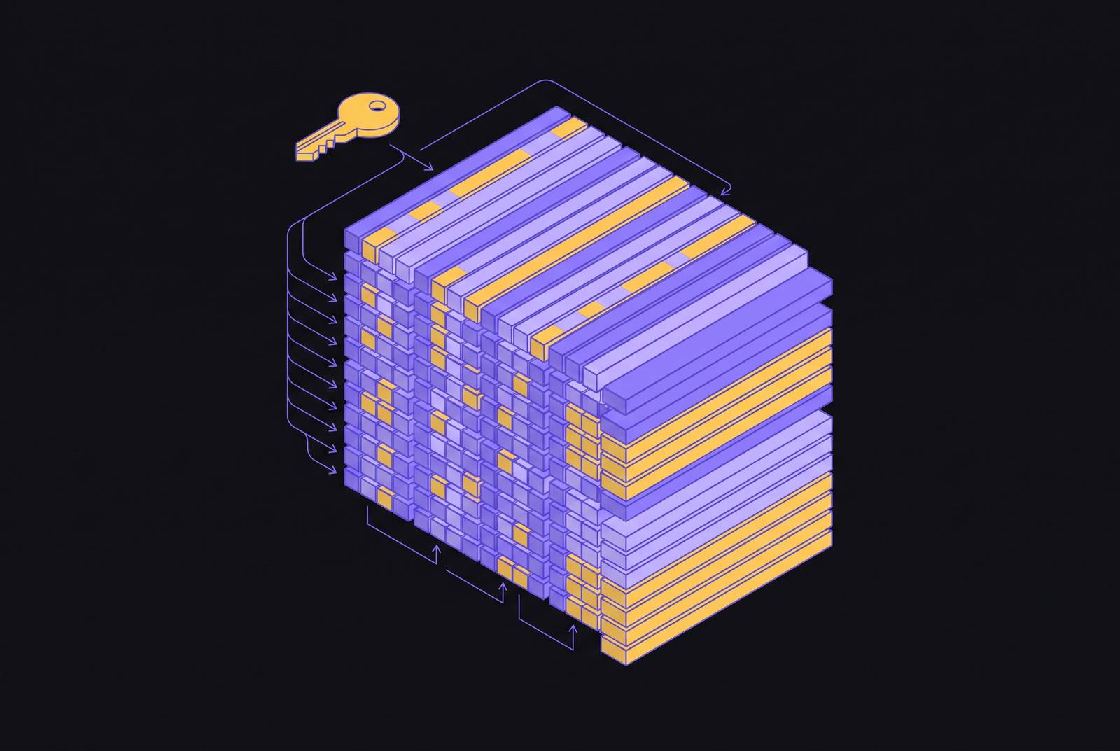
Snowflake has no B-tree indexes, no secondary indexes, and no equivalent of the index tuning that dominates performance work in traditional relational databases. In their place sits a single architectural mechanism: automatic micro-partitioning. Every table Snowflake stores gets divided into immutable, columnar blocks of roughly 50 to 500 MB, and each of those blocks carries its own metadata, including the minimum and maximum value of every column, distinct counts, and additional optimization properties the query optimizer can consult. When a query runs, Snowflake checks that metadata against the query's filters and skips any micro-partition that cannot possibly contain a matching row. That skipping, known as pruning, is the entire performance lever available on a Snowflake table, and it happens automatically with no user action required to make it fire. What determines how well it fires is physical: how tightly rows that share filter values are packed into the same micro-partitions, a property Snowflake calls natural clustering.

This matters most for a specific audience. The tools discussed throughout this piece, clustering keys and the broader clustering machinery, sit on Enterprise Edition and above, and they only become relevant at the scale where pruning efficiency starts to decide query cost rather than query correctness. Teams running large-scale analytical workloads against tables in the terabyte range are the intended audience here, not teams running a handful of gigabytes through a starter warehouse. For those smaller workloads, natural clustering is rarely a problem worth solving, a point the next section explains in more detail.

How natural clustering degrades into a performance problem

Snowflake clusters new data by insertion order by default. For an append-only table loaded in timestamp order, that default is often good enough on its own, because rows that arrive close together in time also land close together on disk. The trouble starts as a table accumulates inserts, updates, and deletes over months or years: that natural ordering degrades, the min/max ranges stored in micro-partition metadata widen, and those ranges start overlapping across more and more blocks. Pruning depends on tight, non-overlapping ranges. Once ranges overlap, the optimizer can no longer rule partitions out with confidence, and it starts scanning blocks it would once have skipped.

The symptom is specific enough to name precisely: a query filtering on a narrow date range ends up touching a large share of the table's micro-partitions, because rows from many different dates have been interleaved across many different blocks through years of incremental writes. Two diagnostic tools surface this condition directly. SYSTEM$CLUSTERING_INFORMATION returns a summary of how well a table's data is organized relative to a given clustering key, including a clustering depth figure that quantifies the overlap. The faster first check sits in the Query Profile itself: comparing PARTITIONS_SCANNED against PARTITIONS_TOTAL for a query with a highly selective filter. If that query is touching a large fraction of the table's total partitions despite asking for a narrow slice of it, natural clustering has failed that workload, and the failure is measurable rather than a hunch about things feeling slow.

This is a large-table problem by its nature. Tables below a meaningful size threshold rarely benefit from any clustering intervention, because Snowflake can scan the entire table in negligible time regardless of how well-organized it is. There's debate about where that threshold should sit: Stellans recommends shortlisting tables over 1 TB as clustering candidates. A sharper framing optimizes for what's actually hot rather than for raw size: a frequently queried 200 GB events table can return more savings per credit spent on clustering than a cold 5 TB archive that gets scanned once a quarter. Stellans's own retail dashboard illustrates the before-state worth diagnosing: a table where queries filtered on transaction date and region were scanning a large share of total partitions, the exact PARTITIONS_SCANNED pathology described above, before any clustering key had been defined.

How to choose clustering columns that improve pruning

Defining a clustering key is a single SQL statement. Choosing the right columns for it is the actual decision, driven by how the table is queried. The columns worth clustering on are the ones that show up in WHERE clauses and join conditions on the table's most frequent or most expensive queries. A clustering key placed on a column nobody filters on does nothing for pruning no matter how cleanly it sorts the data.

Cardinality constrains what will work. Medium-cardinality columns, things like dates, regions, or categories, tend to be the most effective candidates, because their min/max ranges are wide enough to overlap heavily across micro-partitions under natural clustering, yet tight enough once clustered to let the optimizer prune aggressively. High-cardinality columns such as UUIDs or random identifiers already prune reasonably well without intervention, since any single value appears in only a handful of rows scattered thinly across the table. Clustering on a column like that adds ongoing reclustering cost for a gain the table's natural layout was already delivering. Very-low-cardinality columns sit at the opposite extreme: a boolean flag or a binary status column splits the table into at most two groups, which caps the pruning benefit a clustering key on that column alone can ever provide. Such a column can still earn a place as a secondary key paired with a date, tightening pruning within date ranges rather than carrying the pruning load by itself.

Column order inside a multi-column key changes what the key does. Snowflake clusters first on the leading column, then sorts within each of those groups by the next column listed, the same logic a composite sort key follows in a conventional database. The practical rule that follows is to put the column with the broadest filtering coverage first, typically a date truncated to day or month, and add a secondary column such as region or tenant ID to tighten pruning further within those date ranges. Stellans's retail dashboard case follows this logic exactly: queries against the table filtered on DATE_TRUNC('day', transaction_date) and region_id, and the team defined the key as CLUSTER BY (DATE_TRUNC('day', transaction_date), region_id), with the date-truncated expression leading and region narrowing within it.

There's a ceiling on how far this can be pushed. Snowflake recommends no more than three or four columns, or expressions, in a single clustering key, because reclustering overhead grows faster than the pruning benefit beyond that point. A table carries only one clustering key, so the choice of columns has to prioritize whichever query pattern dominates the table's workload rather than trying to serve every possible filter equally. Expressions are valid clustering keys in their own right: DATE_TRUNC('day', event_ts), YEAR(date), and SUBSTRING(product_code, 1, 6) are all legitimate choices when queries consistently apply that same function to the raw column, since clustering on the expression tightens pruning specifically for the queries that use it.

Multi-tenant SaaS tables are a clean application of this same query-driven logic rather than a separate rule to memorize. When nearly every customer-facing query against a table carries a tenant_id predicate, that column, or a compound key pairing it with a date, becomes a natural first candidate, because clustering on it keeps each tenant's rows co-located and keeps scans bounded within that tenant's own micro-partitions. Each case above follows the same rule stated at the top of this section: look at what the queries actually filter on, and cluster on that.

When clustering keys are the wrong tool entirely

Clustering is not a universal performance switch, and treating it as a default setting rather than a precision tool produces bad outcomes in at least three distinct scenarios: write-heavy tables, point-lookup queries, and tables small enough to scan in full regardless of layout.

Write-heavy tables punish clustering through a mechanical fact about how it works. Every insert, update, or delete creates new micro-partitions, and automatic clustering then has to recluster those new partitions to restore order, which consumes credits continuously rather than once. A table whose write pattern resembles OLTP, constant small updates rather than append-heavy batch loads, turns that reclustering bill into something that compounds with every transaction rather than settling into a predictable steady state. The practical test is whether the table changes more than it gets queried: if DML is frequent and unpredictable, steady-state reclustering cost will outrun whatever the query savings deliver. Snowflake's own Well-Architected Framework names frequent DML operations directly as a driver of significant clustering cost overrun.

Point lookups are a different mismatch. A query like WHERE customer_id = 12345 against a massive table is a highly selective equality lookup, not a range scan, and a range scan is the access pattern clustering keys are built to help with. The Search Optimization Service fits equality and substring lookups better, because it builds a separate search-access structure that prunes those filters without physically reordering the table the way a clustering key does. SOS bills its own credits, so it calls for the same cost-benefit scrutiny as clustering does, but for point lookups it typically wins on a per-query basis. Snowflake positions the two as complementary rather than competing: clustering wins on range and date filters that scan a contiguous slice of the table, and SOS wins on lookups scattered across the whole table.

Clustering also interacts badly with layered table structures. Snowflake's documentation recommends clustering at only one level of a table-and-materialized-view hierarchy, since clustering at multiple levels multiplies maintenance cost without a matching multiplication in benefit.

One adjacent fix deserves a direct correction: upsizing a warehouse is not a substitute for clustering. A larger warehouse scans faster, but it does not reduce the number of micro-partitions a query has to scan, because that number is a function of physical layout, not compute size. Warehouse size buys raw throughput. Pruning efficiency is a separate axis entirely, and if PARTITIONS_SCANNED is the actual bottleneck, only clustering or SOS addresses it at the root. Upsizing the warehouse treats the symptom and leaves the cause in place.

Estimating the cost structure of automatic clustering

Automatic clustering is billed through Serverless Credits, a separate pool from the credits a virtual warehouse consumes, and that distinction has a direct accounting consequence: clustering runs in the background independent of warehouse state, so it does not pause when a warehouse suspends and its cost will not show up in whatever dashboard a team uses to watch warehouse spend. A team that only monitors warehouse credit consumption can watch clustering costs accumulate unnoticed.

That cost arrives in two phases that behave very differently and need to be estimated separately. The first pass after a clustering key is defined has to reorganize the table's entire existing history, not just the rows that arrive afterward, and for a large historical table this initial reclustering is often the single largest cost event in the whole project. Snowflake provides SYSTEM$ESTIMATE_AUTOMATIC_CLUSTERING_COSTS specifically to project that cost before committing to a key, and it's worth running before enabling clustering on anything of meaningful size rather than after. Snowflake's own getting-started documentation walks through a worked example in which the function projected roughly 36.6 credits to bring an example table to a well-clustered state, a figure that illustrates the kind of number the function returns rather than a benchmark to expect on any particular table.

Once a table reaches a well-clustered state, a second and smaller cost phase takes over: steady-state maintenance. That recurring cost is driven by table size, the volume of ongoing changes, how far the table's clustering has drifted from ideal at any given moment, and how many columns the clustering key carries. Teams running tables with seasonal or bursty write patterns have a lever available here: ALTER TABLE... SUSPEND RECLUSTER pauses background reclustering and its credit consumption while leaving the key definition in place, which gates cost during a quiet period without forcing a full redefinition later.

The decision that justifies any of this spend is a measurement exercise. The approach that holds up is to compare costs before committing to the ongoing automatic-clustering model against the cost of a one-time reorganization: analytics.today's comparison of INSERT OVERWRITE against standing automatic clustering makes the case that for tables with a known, largely static access pattern, a single pre-sorted load can deliver most of the pruning benefit at a fraction of what continuous automatic reclustering would cost over the same period. That comparison is the right lens for the estimation step broadly: track PARTITIONS_SCANNED, clustering depth, and warehouse credit consumption on the target queries before enabling any clustering mechanism, then take the same measurements after the table stabilizes. Stellans's retail dashboard project followed exactly this before-and-after discipline, measuring average query time and warehouse credit consumption on both sides of the change and confirming a meaningful speed improvement alongside a substantial drop in credit use for the queries that mattered. That measurement discipline is what separates a clustering decision that pays for itself from one that quietly doesn't.

Implementing a clustering key: syntax, initial load strategy, and ongoing monitoring

The syntax itself is the easiest part of this whole process. A new table can declare its clustering key at creation:

CREATE TABLE orders (...) CLUSTER BY (order_date, customer_id);

An existing table takes the key through an ALTER statement:

ALTER TABLE orders CLUSTER BY (order_date, customer_id);

Changing the key later follows the same pattern:

ALTER TABLE orders CLUSTER BY (new_column);

That statement schedules reclustering rather than forcing it immediately. Snowflake's own documentation is specific on this point: changing a clustering key does not affect existing records until the table has actually been reclustered, and Snowflake only reclusters a table if it determines the table will benefit from the operation, so the background process runs on its own schedule rather than on command. A key can also be retained without the ongoing cost:

ALTER TABLE orders SUSPEND RECLUSTER;

That pauses background reclustering and its credit consumption while keeping the key definition intact, useful for a table heading into a known quiet period.

For a large historical table, enabling automatic clustering on a huge, unsorted table before sequencing the work immediately triggers that expensive initial reclustering pass discussed above, reorganizing the table's entire history in one sustained burst of Serverless Credit consumption. The cheaper path front-loads that work using a one-time bulk operation instead: INSERT OVERWRITE... ORDER BY (clustering_key_columns) pre-sorts the table's existing data along the intended clustering columns before automatic clustering is ever turned on. Automatic clustering then only has to maintain an already-reasonable layout going forward rather than build one from scratch, which is the same cost logic behind the INSERT OVERWRITE comparison in the previous section.

Monitoring after implementation is not optional and not a one-time check. The same metrics used to diagnose the original problem, clustering depth from SYSTEM$CLUSTERING_INFORMATION and the PARTITIONS_SCANNED to PARTITIONS_TOTAL ratio in the Query Profile, need to be watched on an ongoing basis against the baseline captured before the key was defined. A clustering key that looked justified at the SYSTEM$ESTIMATE_AUTOMATIC_CLUSTERING_COSTS stage can still drift out of alignment with its workload as query patterns shift, new filter columns become common, or write volume changes shape. Tracking those numbers continuously, rather than trusting the initial decision indefinitely, is what keeps a clustering key doing the job it was defined to do.