Partition Pruning Verification and Micro-Partition Optimization in Snowflake

Partition pruning verification and micro-partition optimization in Snowflake center on one principle. Performance depends on both what the engine can avoid reading and how quickly it processes what remains. Filter, LIMIT, top-k, and join pruning use the same min/max metadata at different points as a query runs. Tuning therefore needs both a data layout that lets pruning work and query profiles that show it did.

Why partition pruning is the dominant lever for Snowflake query performance

Snowflake separates compute from storage, so reading an unnecessary micro-partition carries a network I/O cost before its rows can be evaluated. Pruning avoids that transfer as well as the work of scanning and filtering irrelevant data. In an on-premises row store, skipping data saves disk I/O. In Snowflake, it also avoids inter-node communication overhead and remote-storage latency, which amplify the cost of poor pruning.

Zimmerer et al.’s SIGMOD-Companion 2025 paper identifies scan and filter work as accounting for more than half of processing time in cloud OLAP systems. The sample ORDERS query profile illustrates the concentration of effort, with nearly 95% consumed by a single table scan. When execution is dominated by that stage, warehouse size, concurrency, and SQL structure are secondary to reducing what the scan reads. Pruning targets the work that consumes the time rather than merely supplying more compute to perform it.

How Snowflake stores data as micro-partitions and what metadata each one carries

Micro-partitions are Snowflake’s implicit horizontal storage units, with data stored in columnar format inside each unit. Each has minimum and maximum values for each column, known as zone maps, along with distinct-value counts and other statistics. The cloud services layer holds this metadata independently of the virtual warehouse. Keeping the metadata there lets the engine check which partitions it needs before warehouse nodes read their data.

Take three micro-partitions that each hold a different date range. A date predicate can exclude any partition whose range cannot contain the requested date without inspecting its rows. If the same dates are scattered across all three partitions, their ranges overlap and the metadata excludes less data. Natural load order therefore shapes pruning before an explicit clustering key exists. Bloom filters, approximate set-membership filters, and secondary indexes cover more cases, but all four regimes rely on min/max metadata.

The four pruning regimes: filter, LIMIT, top-k, and join

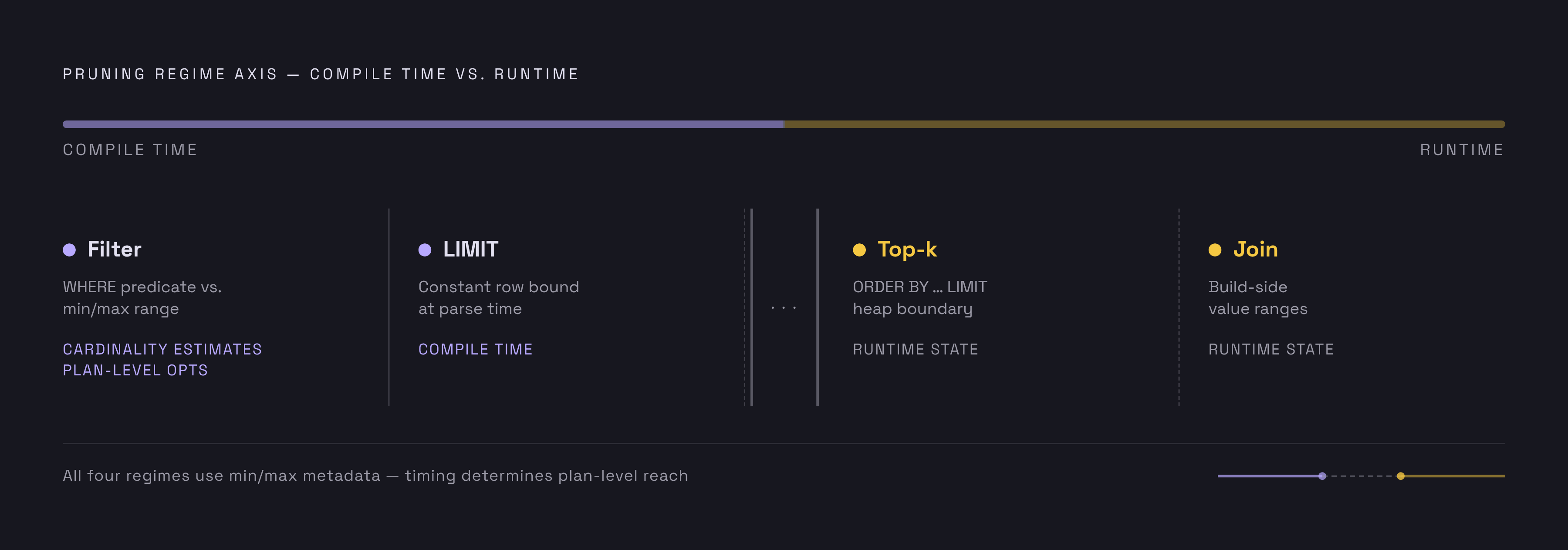
Zimmerer et al.’s SIGMOD-Companion 2025 paper describes four pruning regimes that use min/max metadata at different points in query processing. The important distinction is not the storage unit being skipped, but the information available when the engine decides to skip it. Filter and LIMIT pruning can act at compile time. Top-k and join pruning need state produced during execution.

Filter pruning compares a WHERE predicate with each micro-partition’s min/max range. This regime excludes partitions whose ranges rule out qualifying rows and has the highest absolute pruning ratio of the four. Its compile-time results can also improve the plan before execution begins.

LIMIT pruning applies to LIMIT queries without ORDER BY, with or without a WHERE clause. The engine finds fully matching micro-partitions, which are guaranteed to contain only qualifying rows. It then uses their row counts to identify the minimum set needed to satisfy the limit. It has no need to find which qualifying rows rank highest, as top-k pruning does.

Top-k pruning applies to ORDER BY … LIMIT queries and operates at runtime. As the top-k heap fills, the engine pushes its current boundary down to the table scan. Partitions whose entire min/max range falls outside that threshold can then be skipped. The boundary depends on results the engine has already seen, so compile-time metadata alone cannot tell it what to skip.

Join pruning also operates at runtime, but derives its bounds from the build side of a join. The engine collects build-side value ranges and excludes probe-side micro-partitions that cannot contain a matching partner. Because those ranges emerge during execution, this pruning cannot influence earlier join-order decisions. By contrast, compile-time pruning can improve cardinality estimates and support sub-tree elimination, constant folding, and other cost-based plan choices.

What the pruning ratios across the four regimes reveal about real workloads

Zimmerer et al.’s paper reports that filter pruning removes the vast majority of micro-partitions across representative customer samples. LIMIT, top-k, and join pruning also eliminate large fractions of the work in their applicable query sets. These findings make the runtime regimes material performance mechanisms. They also show why evaluating pruning only through selective WHERE clauses leaves out meaningful gains.

The same paper finds that production analytical queries are much more selective than common benchmark assumptions suggest. TPC-H does not reflect those production distributions and therefore understates the value of pruning improvements. A partition scan count that looks acceptable on synthetic data is not a reliable forecast for a production workload. Benchmark results must therefore be distinguished from evidence about the predicates and distributions a table actually serves.

How clustering keys shape which micro-partitions each regime can skip

Clustering places rows with similar key values together, narrowing the min/max ranges within individual micro-partitions. A filter can reject more ranges, a join can rule out more probe-side partitions, and a top-k boundary can exclude more of the remaining scan. Clustering changes the precision of the metadata rather than changing the underlying pruning mechanism.

The unclustered LINEITEM example illustrates the failure mode by scanning every micro-partition before clustering was applied. When predicate values are scattered throughout a table, metadata cannot establish that a partition is irrelevant merely because the query is selective. Natural clustering can provide the needed separation without explicit maintenance when data arrives in time or key order. Snowpipe streaming ingest can disrupt that order by interleaving rows from different key ranges.

Clustering also benefits the read side of WHERE-filtered DELETEs and UPDATEs by reducing the partitions that must be scanned. However, DML creates new micro-partitions and can degrade clustering over time. Putting the layout back in order through reclustering then takes more writes.

When clustering adds cost without adding enough pruning benefit

Automatic clustering is not a universal improvement because its credit consumption scales with the volume of data reorganized. On a frequently changing table, repeated maintenance may cost more than the queries save. Snowpipe ingest can compound that expense when incoming rows continually disrupt key order. Tables occupying only a handful of micro-partitions have too little pruning opportunity to justify the overhead.

A poorly chosen key creates a different imbalance. It may produce tight ranges on columns that common queries never filter, while leaving the relevant scans largely unchanged. The table then incurs reorganization cost without receiving the intended read benefit. Clustering health alone is consequently not proof that the key serves the workload.

The practical test is to compare clustering credits spent with query credits saved over the same window. AUTOMATIC_CLUSTERING_HISTORY provides the maintenance side of that comparison. The choice to turn on automatic clustering across large or frequently updated tables must weigh that ongoing cost alongside the speed of an example query. The unit of judgment is the table and its workload.

How to confirm pruning fired: reading the query profile and system functions

Checks start with the health of the clustering before the query runs. SYSTEM$CLUSTERING_INFORMATION reports clustering depth and overlap for candidate columns or the table’s defined clustering key. High average depth or overlap indicates that similar key values span many partitions, predicting weaker pruning. This establishes whether the physical layout supports the intended predicate, but it does not establish what a particular execution skipped.

After the query runs, look at the query profile’s Table Scan node and compare partitions scanned with partitions total. A small scanned fraction shows that the query avoided much of the table. A near-total scan on a query expected to be selective calls for examination of the key, the data layout, and the predicate expression. Those statistics connect the proposed optimization to the work actually performed.

Snowflake’s well-architected performance guide identifies the query profile’s “Most Expensive Nodes” section as a way to locate dominant execution work. When Table Scan dominates and partition scan counts are high, pruning is the bottleneck. The plan may show some static filter and LIMIT decisions, but it alone cannot show how much work was saved at runtime. Top-k and join pruning require post-execution statistics, and runtime filter pruning is likewise not fully represented by the compile-time plan.

Where column expressions defeat min/max pruning and what Optima Metadata does about it

Even with healthy clustering, pruning can fail because zone maps hold raw stored values and lack the results of arbitrary expressions. A predicate such as WHERE UPPER(email_domain) = 'SNOWFLAKE.COM' cannot be evaluated against the raw column’s min/max values through standard pruning. Similar gaps arise with LOWER(), TO_DATE(), and ILIKE patterns containing leading wildcards. Narrowing the raw ranges does not supply the missing information about transformed values.

A cybersecurity search can use ILIKE '%connection timeout%'. The query looks for a phrase within a value, while the standard zone map holds the column’s minimum and maximum. Those bounds do not establish which partitions can contain the phrase. Treating this expression-evaluation gap as a clustering defect would target the layout.

Snowflake Optima Metadata, released January 2026, addresses that gap by analyzing query history for frequently used expressions. It generates lightweight, expression-specific metadata autonomously, with no configuration, no extra cost, and no manual intervention required. Teams therefore do not need to predict which expressions will become hot before the workload develops. When an expression becomes infrequent, Optima Metadata removes its custom metadata automatically.

A practical decision sequence: from new table to verified pruning

Inspect the most frequent and most expensive queries to identify the WHERE, JOIN, and ORDER BY columns that dominate their access patterns. Those columns show which keys to try and which pruning regimes should gain from them. Without that connection, even an orderly table can be organized around the wrong values.

Next, run SYSTEM$CLUSTERING_INFORMATION on the candidate key to assess natural clustering. Ordered loads may already have ranges narrow enough for pruning, so automatic clustering would cost more without helping queries skip more data. Where they do not, enable clustering selectively for large tables with sufficiently stable data and matching query patterns. Use AUTOMATIC_CLUSTERING_HISTORY to compare what maintenance costs with what it saves on queries.

Then run the relevant queries and inspect their partition scan counts, using post-execution statistics for top-k and join pruning. If clustering looks healthy but scans still read much of the table, check whether the predicates transform columns before blaming the choice of key. Finally, re-verify after schema changes, ingest changes, or major DML operations, using periodic SYSTEM$CLUSTERING_DEPTH checks to catch layout regressions. Pruning is a property of the current workload and data arrangement.

How these pruning principles apply when Snowflake is the destination in a SaaS data pipeline

For product teams delivering data into customer-owned Snowflake warehouses, the load architecture shapes downstream pruning. Arbitrary row order can widen ranges on time or key columns and shift the resulting cost to the customer. That customer must then let queries scan more data or pay for reclustering to put it back in order. Batch loads sorted on the primary query predicate column, however, can give natural clustering that helps pruning without the customer having to configure clustering.

Destination schema design also affects what metadata can prove. Landing columns that queries routinely filter through UPPER(), ILIKE, or date conversions introduces the expression-pruning gap, even when the load order is sound. Pre-computing canonical forms before loading is one way around that gap, while Optima Metadata creates expression-specific metadata on its own. These choices connect data delivery directly to the destination’s scan behavior.

For teams embedding data export as a product feature, successful delivery is therefore not the whole performance boundary. The choice of batch or streaming delivery, the order of rows, and the destination schema affect how much work the customer’s queries do and what maintenance costs. The same pruning principles apply whether the warehouse belongs to the vendor or the customer. Destination-side performance follows from both how data arrives and what the executed query profile shows it can skip.